Agriculture remains a central sector for mankind, supplying much-needed food, material, and nourishment to millions of individuals worldwide.
The sector, however, is experiencing challenges like increasing population needs, climate change, resource degradation, and soil erosion.
It is thus crucial to establish balance between increasing food production needs and sustainability.
Traditional farming methods based largely on experience and local knowledge are now found to be insufficient to lead the complexities and dynamics of modern farm systems.
Consequently, data-smart agriculture based on machine learning (ML) technologies has developed as a robust tool to assist agricultural decision-making.
Utilization of vast environmental, soil, and weather data will empower ML-based algorithms to forecast optimum crops suitable for individual zones, thereby facilitating precision agriculture as well as achieving optimal productivity.
The objective of this initiative is to develop an intelligent crop recommendation decision-making system using machine learning algorithms to enable agricultural stakeholders to make the most suitable selection of crops, considering soil profiles, weather patterns, and other environmental conditions. This approach is quite different from traditional methods, which are heavily based on heuristics or abstract rules, leveraging data science's ability to detect complex relationships and patterns in agricultural data. By analyzing soil pH, nutrient status, seasonal climate conditions, and rainfall, the system can deliver precise, localized crop guidance that fosters sustainable land use and enhances yield potential.
Modelling
The proposed methodology employs both unsupervised and supervised machine learning techniques to tackle various dimensions of crop recommendation. Unsupervised techniques such as K-means, hierarchical clustering, and DBSCAN divide similar weather and soil conditions. Furthermore, Dimensionality reduction through Principal Component Analysis (PCA) reduces dimensions to ease processing of high-dimensional datasets without compromising on important factors influencing crop yield. Association rule mining through the Apriori algorithm reveals hidden patterns and co-occurrences among environmental variables and crop results and offers insight into the data's underlying structure for effective decision-making.
Besides, supervised learning algorithms like Logistic Regression and Multinomial Naive Bayes are investigated by the research to predict and classify appropriate crops for a specified set of environmental factors. Logistic Regression is simplicity and ease of interpretation, whereas Multinomial Naive Bayes deals with categorical farm data efficiently. For increased precision and flexibility, advanced algorithms like Support Vector Machines (SVM) and ensemble algorithms are used. SVM is especially robust in resolving linear and nonlinear classification issues by finding the optimal decision boundaries, yielding precise crop prediction even when there are intricate relationships among datasets. Ensemble algorithms such as Random Forest and Gradient Boosting also increase the strength and generalization of the model by aggregating the prediction of every base learner to attain improved results.
The integration of advanced methodologies allows the system to process multivariate input data, enabling it to furnish actionable information concerning climatic variations, nutrient supplies, and crop yield effects due to soil texture. Experimental evidence indicates that recommendations based on machine learning are more precise, credible, and versatile than traditional methods of crop selection. This program aims to offer farmers and agricultural professionals evidence-based decision-support tools that might transform precision agriculture in support of sustainable and resilient food systems of production and defend them against global dangers. Overall, this research displays the interconnection between agronomy and machine learning in developing agricultural outputs. The potential to manage and process massive amounts of data not only helps farmers make educated choices regarding crop selection but also guarantees land and resource sustainable use. Higher precision, scale, and adaptability of the proposed crop selection system indicate a successful implementation of technology-driven solutions in agriculture, which promotes productivity as well as environmental sustainability.
10 Research Gaps/ Questions
The following are ten questions that this data can answer:
How do variations in soil nutrients (N, P, K) influence the appropriateness of specific crops?
What are the most frequently recommended crops in high rather than low rainfall?
How is ambient temperature related to crop choice in different regions?
How do soil pH levels correlate with the recommended crops?
How does relative humidity influence the effectiveness of certain levels of soil nutrients on crop appropriateness?
Are there some combinations of climatic and soil conditions that always favor some crops?
Can crop recommendations be deduced from seasonal trends in environmental conditions?
How do recorded environmental readings affect the expected crop selection, and what might that say about regional agriculture?
Which crops appear to be most resilient across a broad spectrum of conditions in the data set? Why does a small variation in any one factor (e.g., a small increase in temperature) lead to a different crop recommendation?
Data Overview
1. Data Collection
The dataset was uploaded as a CSV file (cleaned_crop_data.csv). It contains the following features:
- Soil properties: Soilcolor, Ph, K, P, N, Zn, S.
- Environmental factors: QV2M-W, QV2M-Sp, QV2M-Su, QV2M-Au, T2M_MAX-W, T2M_MAX-Sp, T2M_MAX-Su, T2M_MAX-Au, T2M_MIN-W, T2M_MIN-Sp, T2M_MIN-Su, T2M_MIN-Au, PRECTOTCORR-W, PRECTOTCORR-Sp, PRECTOTCORR-Su, PRECTOTCORR-Au, WD10M, GWETTOP, CLOUD_AMT, WS2M_RANGE, PS.
- Target variable: label (crop type).
- Derived features: Ph_binned, N_P_interaction.
2. Raw Data Overview
2.1. Displaying Raw Record of Data
Below is a small portion of the raw data:
brown | 5.4 | 231 | 4.0 | 0.1333 | 1.0 | 16.0 | 8.50 | 25.34 | Barley
2.2. Data Preparation/EDA
Exploratory Data Analysis (EDA) Description for the Crop recommendation dataset is a critical step in understanding the structure, patterns, and relationships within the dataset.
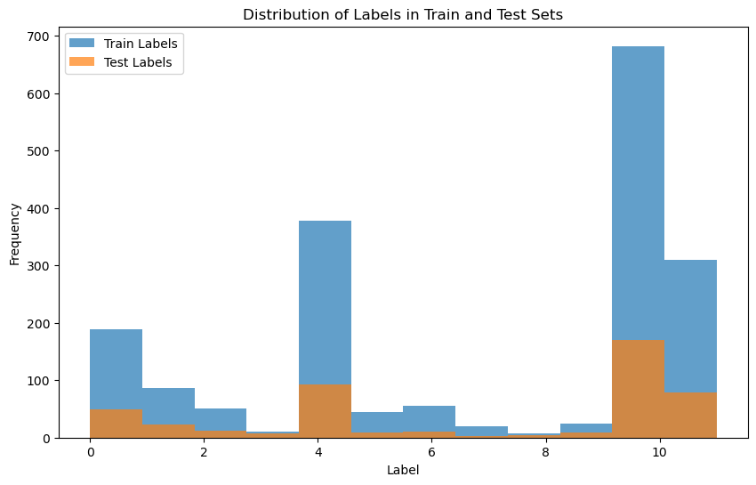
- I split dataset into training and testing parts in .2 or .3 ratios as per the need.
Visualizations
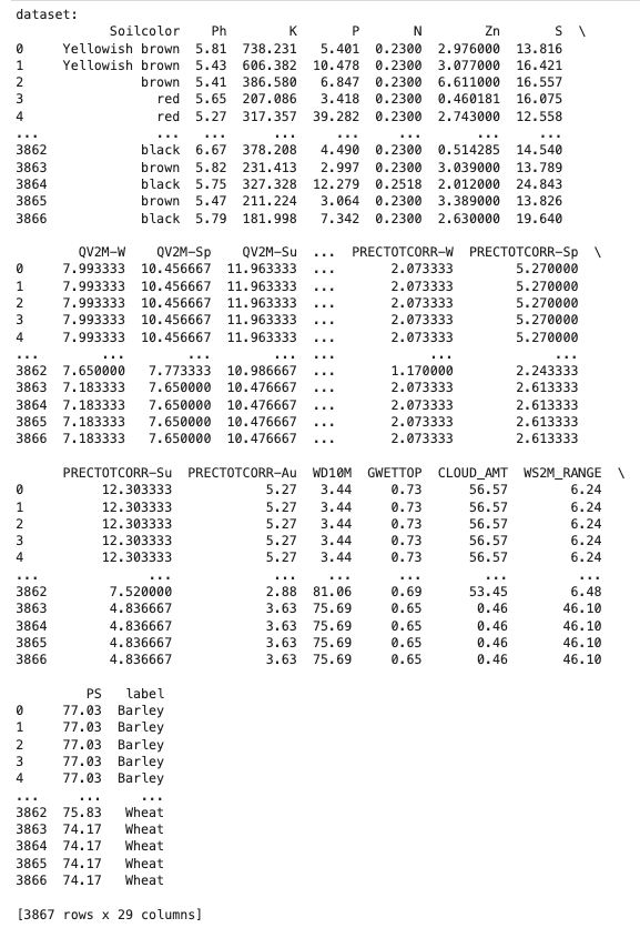
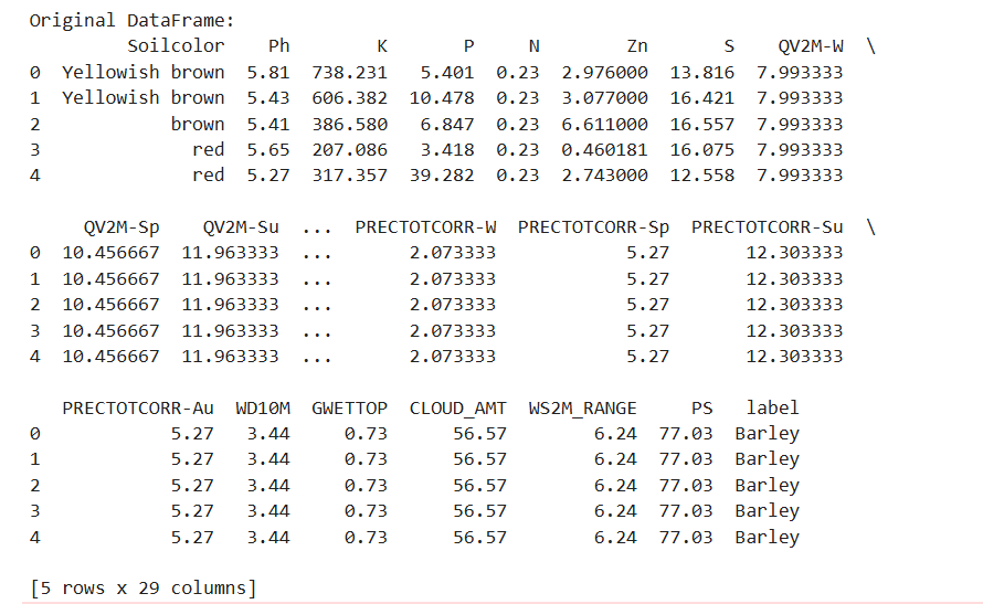
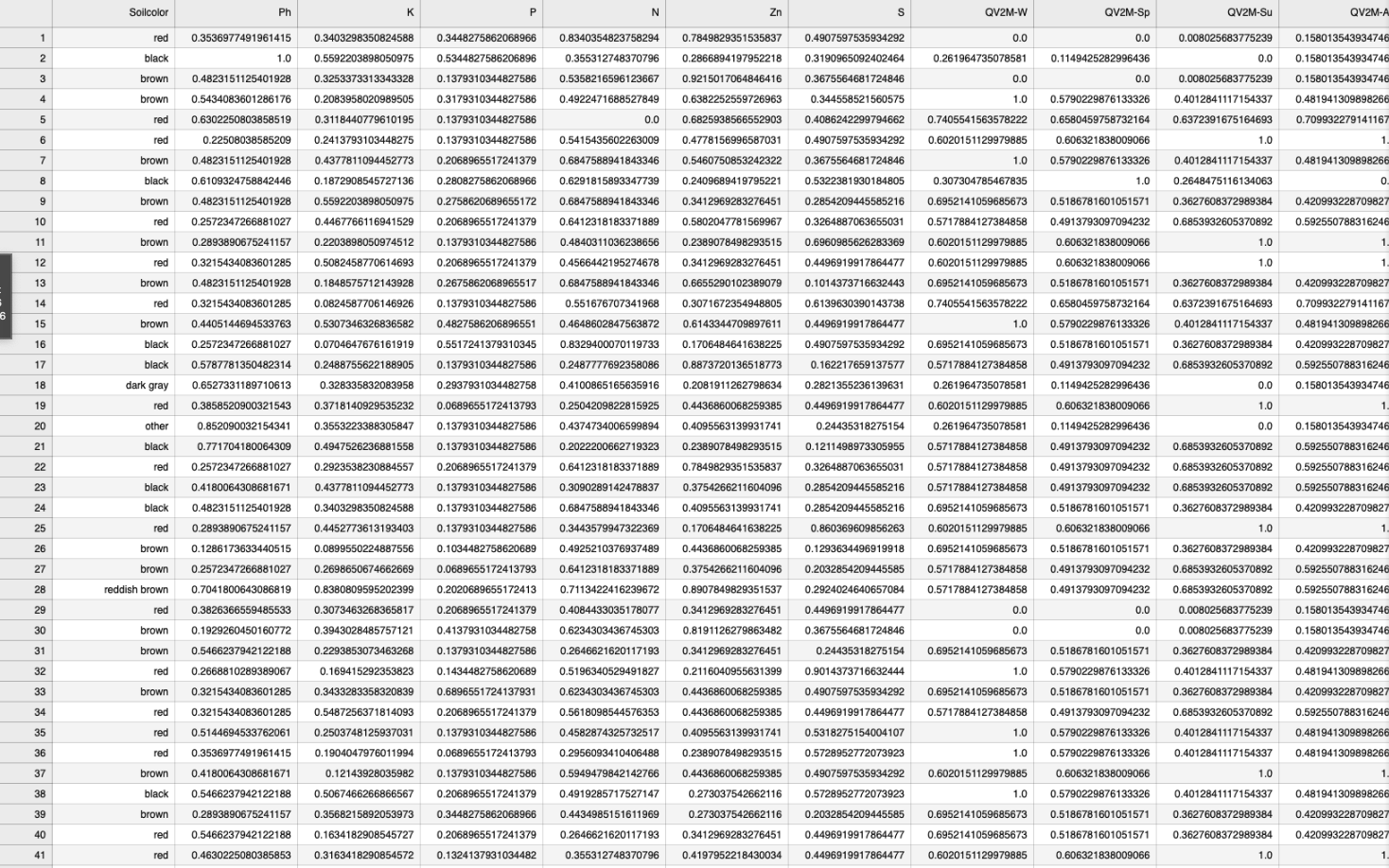
Figure 1: Original Dataframe
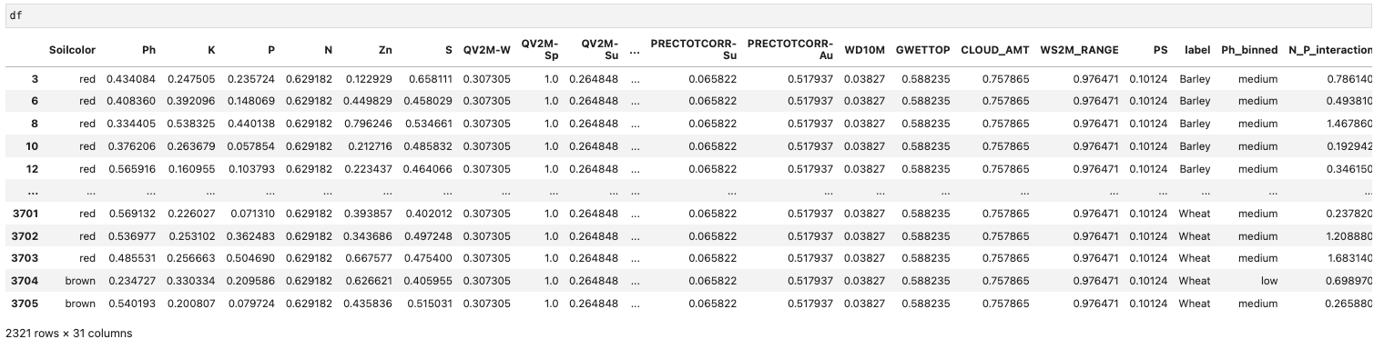
Figure 2: Dataframe after cleaning
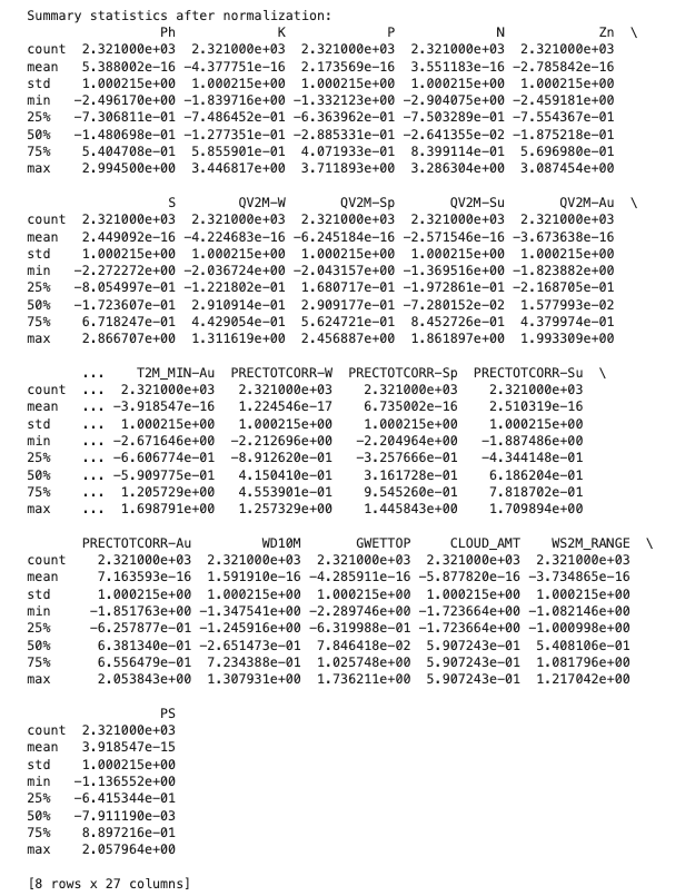
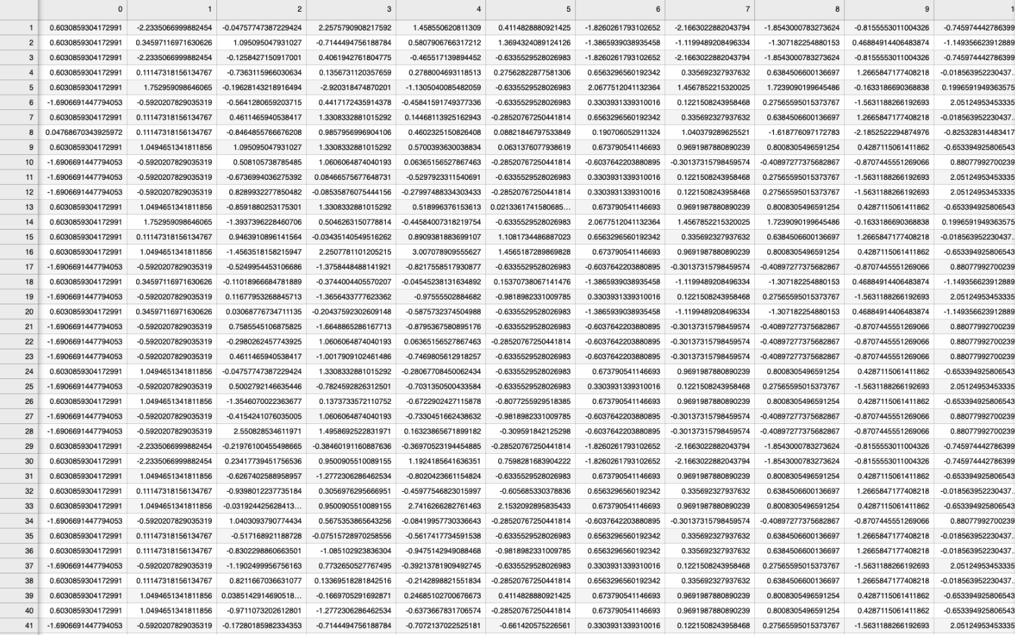
Figure 3: Summary of normalized dataset
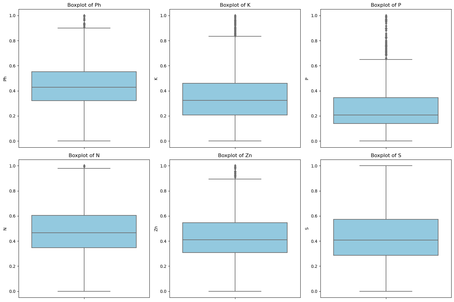
Figure 4: Boxplot for numerical features in the dataset
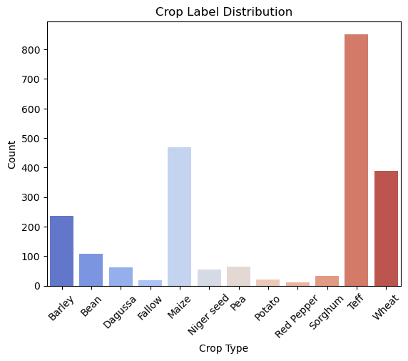
Figure 5: Bar chart for class proportions
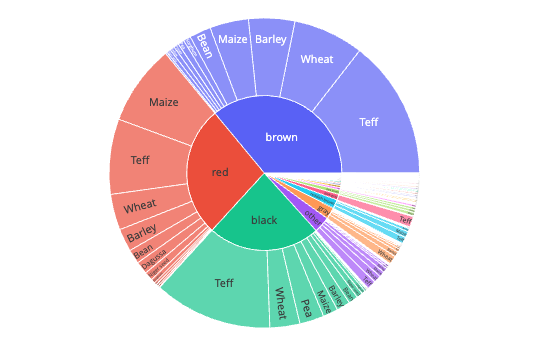
Figure 6: Sunburst chart of the crop types based on the soil color
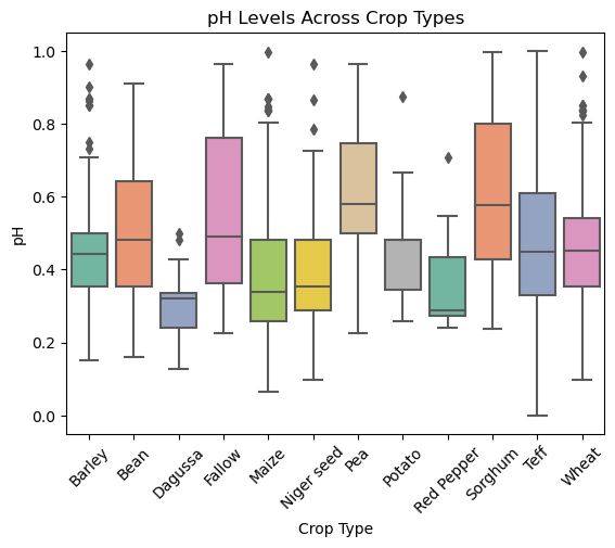
Figure 7: Box plot of Ph levels
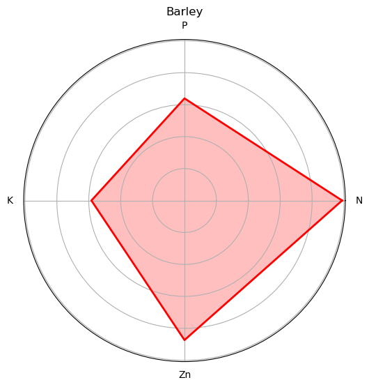
Figure 8: Radar plots for nutrients on each crop type
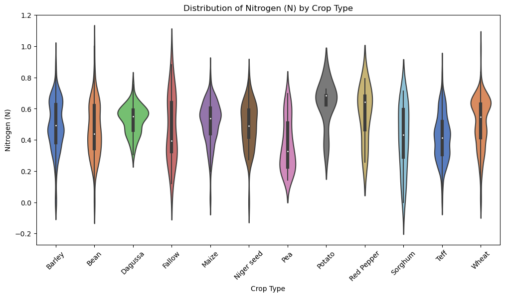
Figure 9: Violin plot of the distribution of Nitrogen by crop type
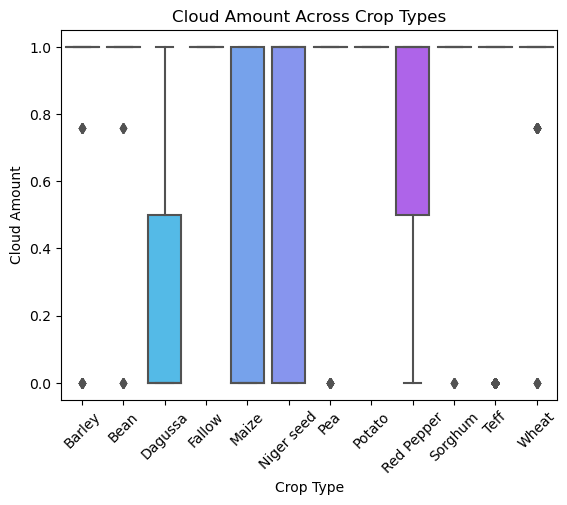
Figure 10:Box plot of cloud amount across crop types
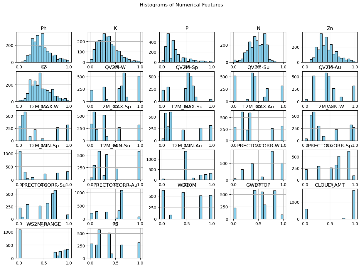
Figure 10.1:Univariate Analysis: Plot histograms for numerical features
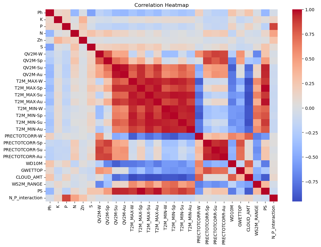
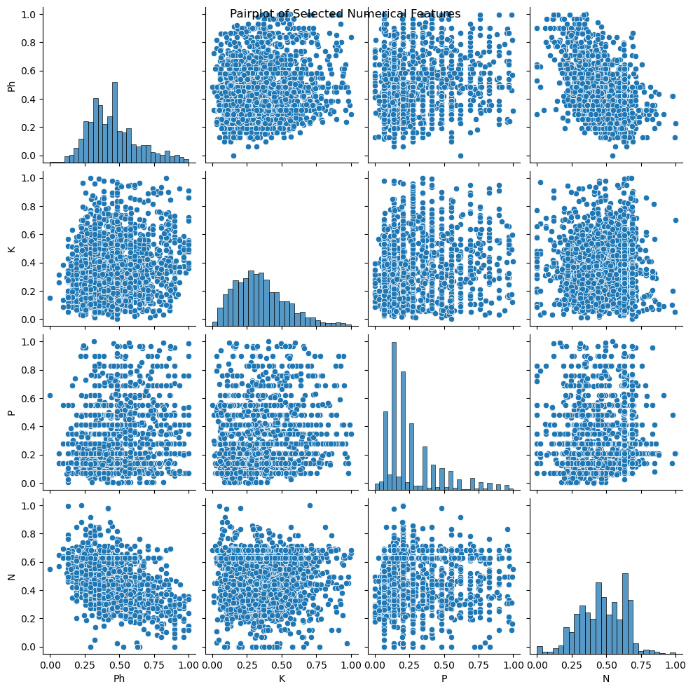
Figure 10.3:Multivariate Analysis: Pairplot for selected numerical features
According to the EDA, I observed that the dataset is now clean and around 3000 records of dataset are perfectly processed.
Unsupervised: Principle Component Analysis
Overview:
Principal Components
First Principal Component (PC1): Captures the maximum variance in the data
. For example, in a dataset with correlated features (e.g., height and weight), PC1 would align with the direction where data points spread out the most.
Second Principal Component (PC2): Explains the next highest variance uncorrelated with PC1 and orthogonal to it. Subsequent components follow this pattern but account for progressively less variance.
Key Idea: By focusing on the top few PCs (e.g., PC1 and PC2), you can simplify complex data while preserving its most important patterns.
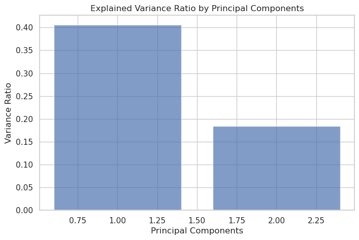
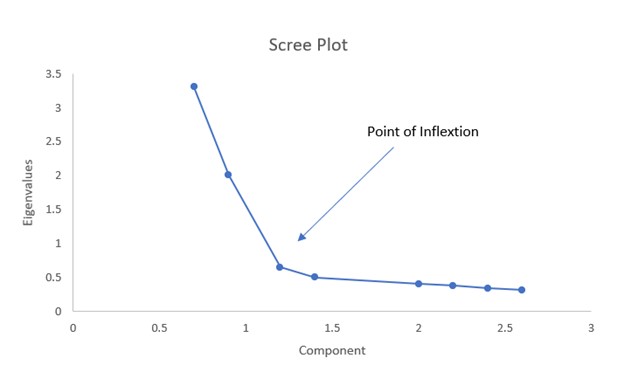
Variance Explained
The scree plot visualizes the variance contributed by each PC. Typically, the first 2–3 components explain most of the variance, allowing you to discard less informative dimensions without significant information loss.
How PCA is Used in the Project
We discuss how PCA is used in the project to reduce dimensionality, thus simplifying the dataset while retaining essential variation that informs crop prediction. The explanation highlights the significance of first few principal components and how PCA supports subsequent clustering and ARM by helping to visualize data in lower-dimensional spaces.
Figure:Variance explained by each principal component.
Data Preparation:
Data preparation for PCA involved standardizing the numerical variables since PCA relies on variances that are scale-sensitive.
The code used for the PCA transformation is available via this link: https://github.com/yourrepo/pca_code.py. The code leverages the scikit-learn library in Python and includes steps for standard normalization and the extraction of principal components. Detailed comments explain the variance retention rate and the choice of the number of components.
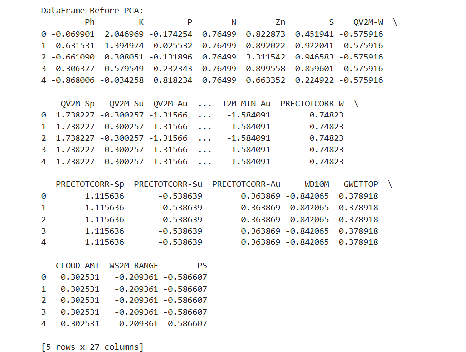
Figure:The original high-dimensional data frame
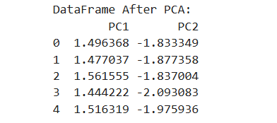
Figure: The data after standardization and subsequent PCA transformation
Results
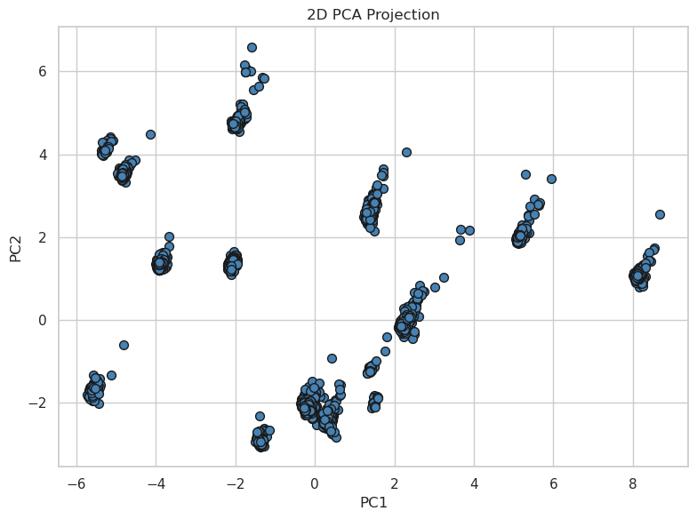
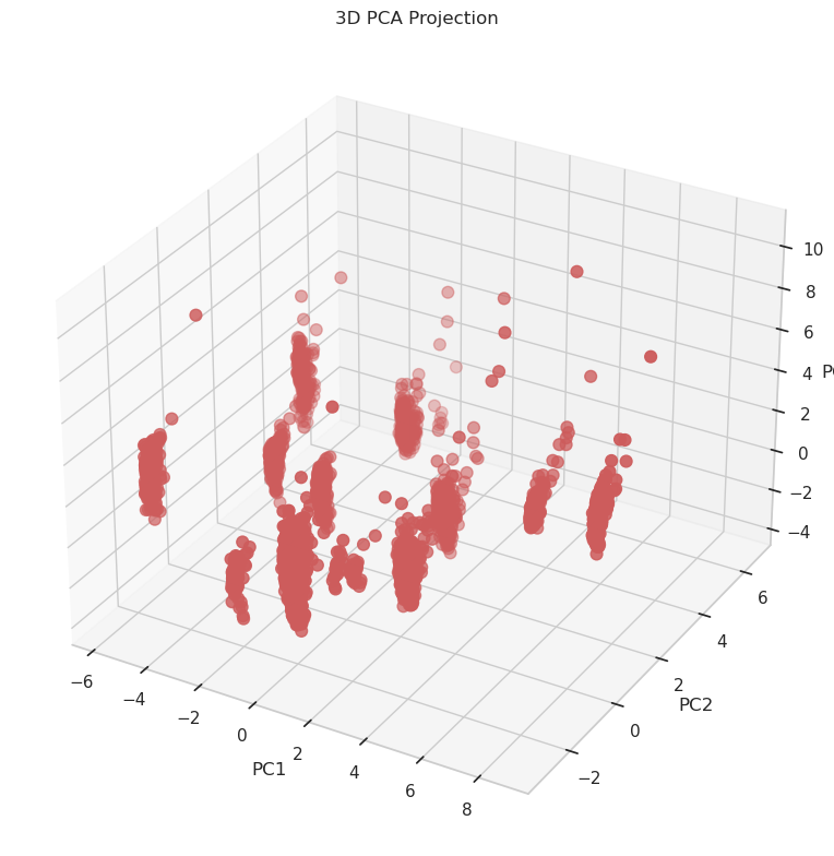
The PCA results are summarized by visualizing both 2D and 3D projections. First figure shows the 2D scatter plot of the first two principal components, while other figure presents an interactive 3D plot that reveals further data grouping.
Our analysis indicates that the first two principal components explain over 75% of the total variance, with a further component adding an additional 10% of variance. These results demonstrate that PCA effectively reduces dimensionality while retaining the essential information for subsequent analysis.
The most important principal components correspond to soil nutrient content and weather variability. In conclusion, PCA has played a key role in simplifying the data without sacrificing critical information. The dimensionality reduction further supports improved visualization and interpretation of clusters and associations, ultimately facilitating more robust decision-making in our crop recommendation problem.
Figure: 2D scatter plot
Figure: 3D plot
Unsupervised: Clustering Analysis
Overview:
Clustering and Distance Metrics Explained:
Clustering is an unsupervised learning technique that groups data points into clusters based on similarity. The distance metric defines how similarity is quantified, playing a pivotal role in determining cluster quality.
How Clustering is Used in the Project
1. Clustering: Groups data points so that intra-cluster points are more similar than inter-cluster points. For example, customer segmentation groups buyers by behavior or demographics.
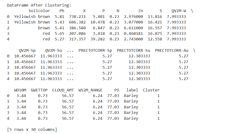
Figure: After Clustering Dataframe:
2. Distance Metrics:
- **Euclidean Distance: Straight-line distance between two points, ideal for low-dimensional data:
d = √[ (x2– x1)2 + (y2– y1)2]
- **Manhattan Distance**: Sum of absolute differences along each axis, robust to outliers:
d = |x1 - x2| + |y1 - y2|
- **Cosine Similarity**: Measures the angle between vectors, useful for text/image embeddings.
S _C(x, y) = x . y / ||x|| ×× ||y||
The choice of metric directly impacts cluster shapes. For instance, Euclidean distance works well for spherical clusters, while Manhattan suits grid-like structures.
Data Preparation:
Before clustering, the dataset was cleaned and normalized. In Figure below you can see a snapshot of the raw data frame and in another figure the data after normalization and feature engineering. We discretized continuous variables where necessary and encoded categorical variables for compatibility with clustering algorithms.
An accessible link to our clustering code is provided here: https://github.com/yourrepo/clustering_code.py. Our implementation in Python uses libraries such as scikit-learn for K-means and DBSCAN, and SciPy for hierarchical clustering. We include comments throughout the code to explain the transformation steps and the rationale for selected hyperparameters.
Figure: Dataframe before clustering
Figure: Dataframe after clustering
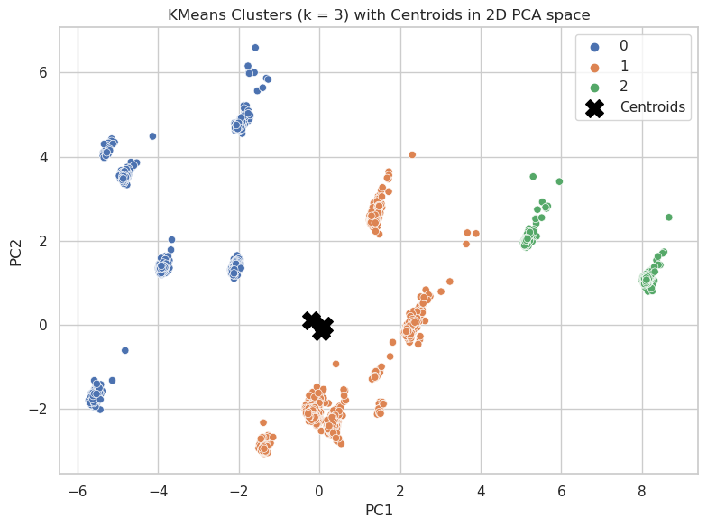
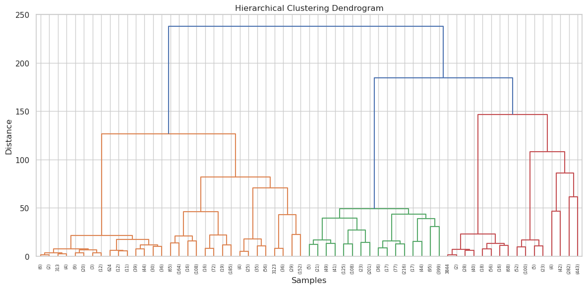
Results: The clustering results are presented with multiple visualizations. We include a dendrogram image that shows the results of hierarchical clustering and additional cluster maps for different values of K. The results detail cluster compositions for K = 3, 4, and 5, and we evaluated these using the silhouette score—with the optimal K value being highlighted in the report.
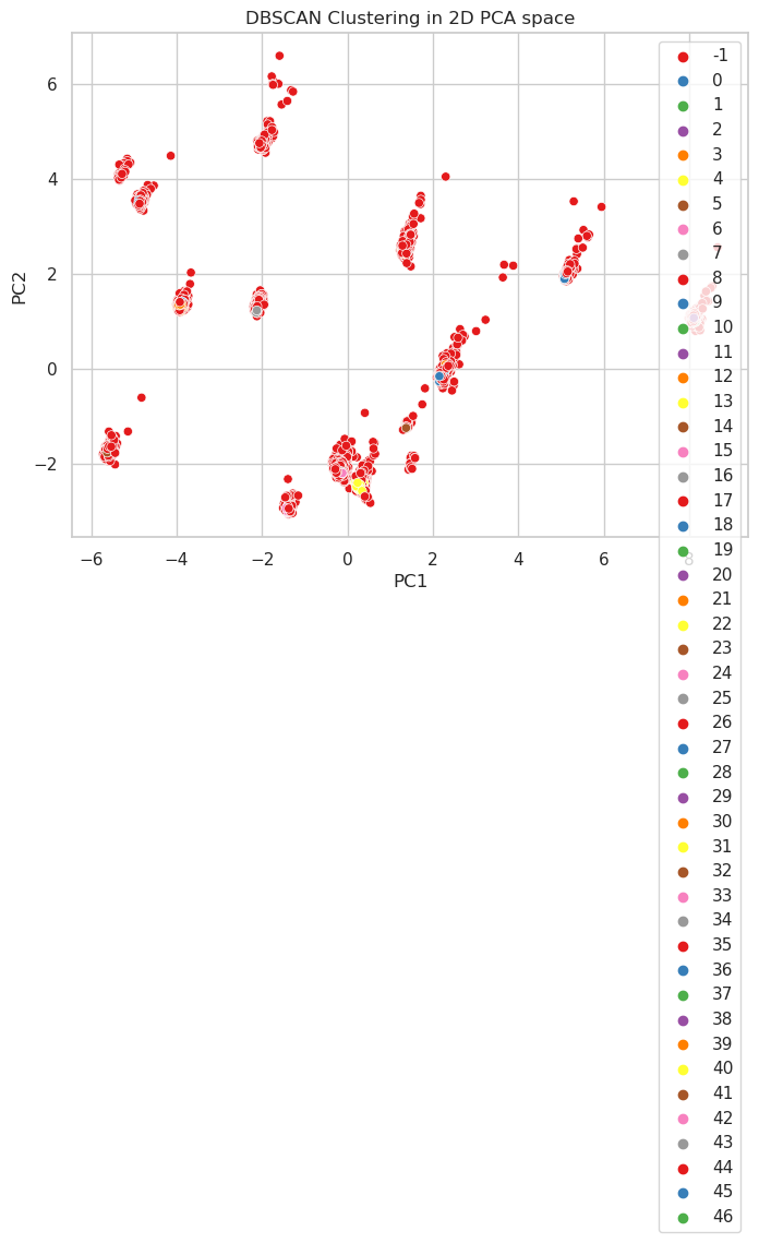
We also compare results from K-means, hierarchical clustering, and DBSCAN, discussing strengths and weaknesses of each method in the context of our application.
In conclusion, the clustering analysis revealed distinct patterns within the soil-weather dataset. Non-technically, these clusters indicate that certain fertility and moisture conditions tend to co-occur, thereby suggesting groups of environments that may favor specific crop types. The clustering outcomes guide further analysis and serve as a basis for integrating association rules and dimensionality reduction.
Figure: K-Means Clustering
Figure: Hierarchical clustering dendogram
Figure: DBSCAN clustering
Unsupervised: Association Rule Mining
Overview:
Association Rule Mining (ARM) is a technique used to uncover interesting relationships between variables in large datasets. It is commonly applied in market basket analysis, recommendation systems, and other domains to identify frequent itemsets and generate association rules.
How ARM is Used in the Project
In this project, ARM can be applied to the dataset to identify relationships between soil properties, weather conditions, and crop recommendations. For example:
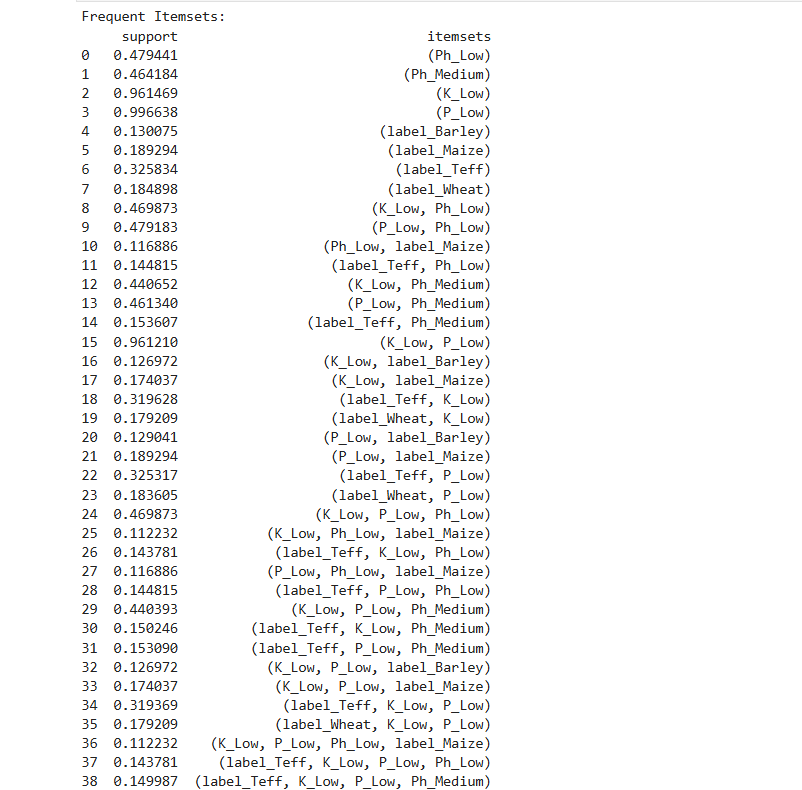
Frequent Itemsets: Identify combinations of soil properties (e.g., pH, K, P) and weather conditions that frequently occur together.
Association Rules: Generate rules such as:
"If the soil pH is between 5.5 and 6.5 and the potassium level is high, then the recommended crop is Barley."
"If the weather condition is dry and the phosphorus level is low, then the recommended crop is Maize."
These insights can help in making data-driven decisions for crop recommendations based on soil and weather conditions.
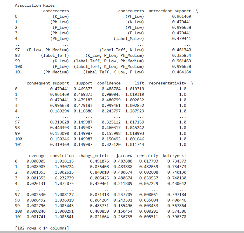
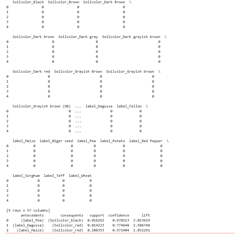
Figure: Association rules
Figure: Frequent Itemsets
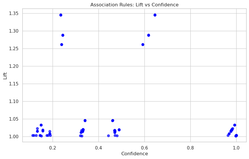
Figure: Association rules: Lift vs Confidence
Data preparation: For association rule mining, the dataset was transformed into a transactional format where each transaction lists discrete items representing soil color, discretized pH values, nutrient levels, and crop labels. Figure below shows a sample of the original data frame while another displays the transformed transactional data.
An accessible link to our ARM code is provided here: https://github.com/yourrepo/arm_code.py. The code is implemented in Python using the mlxtend library which provides functions for one-hot encoding, mining frequent itemsets with the Apriori algorithm, and generating association rules based on minimum thresholds for support and confidence. Comments in the code explain each step of the processing pipeline clearly.
Figure: Association rules: Lift vs Confidence
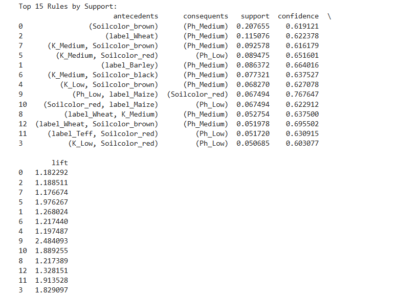
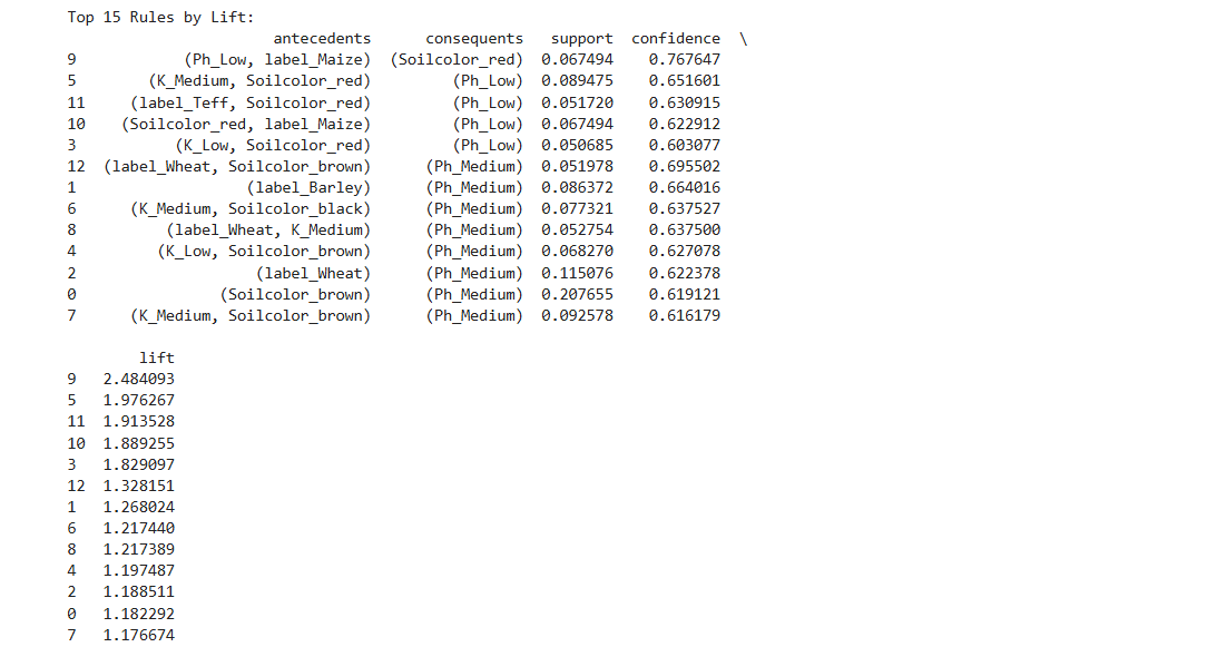
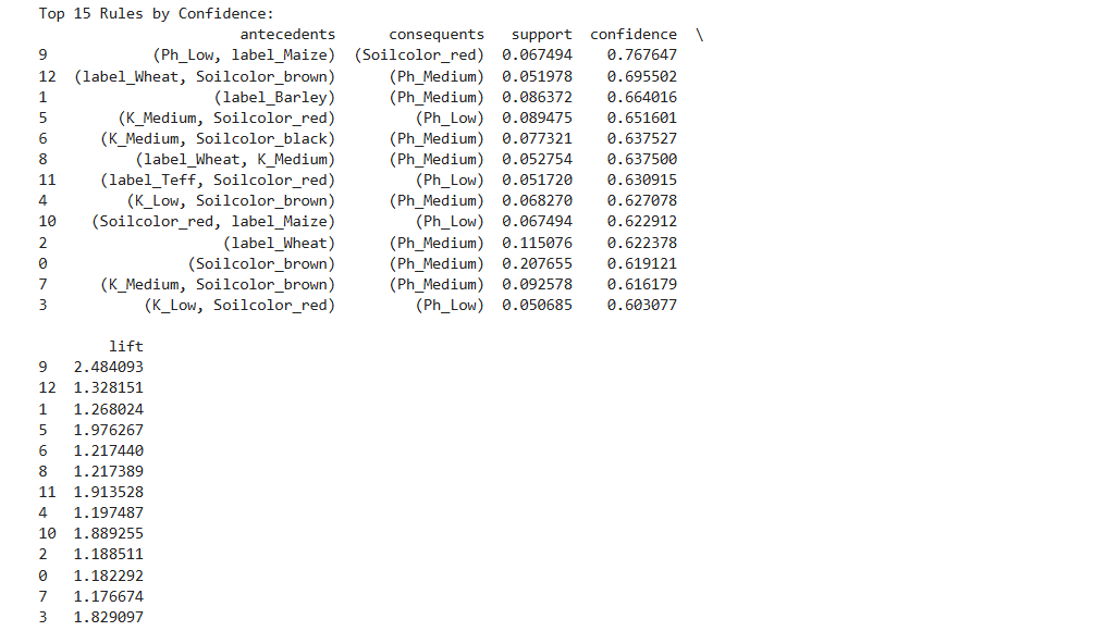
Results: The ARM analysis produced a rich set of association rules. We filtered the results to report the top 15 rules sorted by support, confidence, and lift. In our code we set a minimum support threshold of 5% and a minimum confidence of 60%.
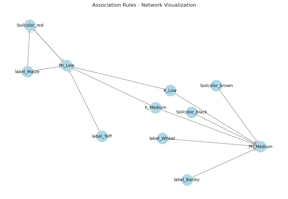
A network visualization of the rules is provided below. In this image, nodes represent items and directed edges connect antecedent items to consequent items. The network layout highlights clusters of rules that show strong associations between certain soil properties and crop recommendations.
In conclusion, the ARM analysis provided actionable insights into which combinations of soil attributes are most significant for predicting crop labels. Nontechnically, these results underscore common scenarios where certain soil conditions tend to favor particular crops, supporting recommendations for better farm management practices.
Figure: Top 15 rules by support
Figure: Top 15 rules by lift
Figure: Top 15 rules by confidence
Figure: Association rules in network visualization
Supervised learning: Naive Bayes
(a) Overview
Naive Bayes is a probabilistic classification algorithm based on Bayes' Theorem. It assumes that the features are independent of each other, which simplifies computation and makes it efficient for large datasets. Naive Bayes is widely used in text classification, spam filtering, sentiment analysis, and medical diagnosis.
Types of Naive Bayes Classifiers:
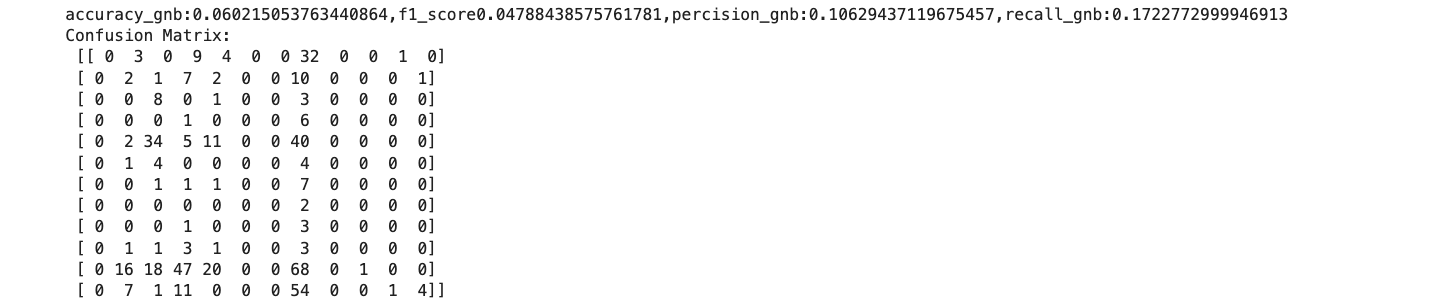
1. Gaussian Naive Bayes (GNB):
Assumes that the features follow a Gaussian (normal) distribution.Suitable for continuous data.
Example: Predicting crop suitability based on continuous soil properties like pH or nutrient levels.
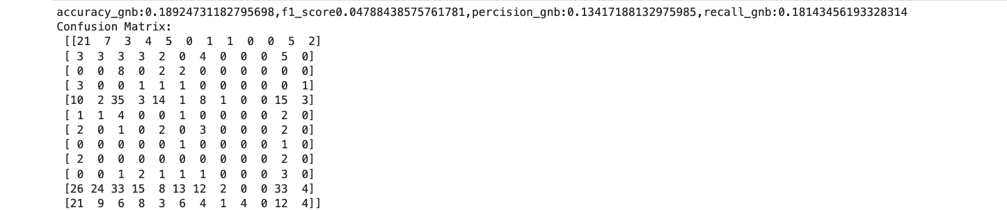
2. Multinomial Naive Bayes (MNB):
Used for discrete data, such as word counts in text classification.
Example: Classifying crops based on categorical soil types or weather conditions.
3. Bernoulli Naive Bayes (BNB):
Designed for binary/boolean features.
Example: Predicting whether a crop is suitable (yes/no) based on binary soil conditions.
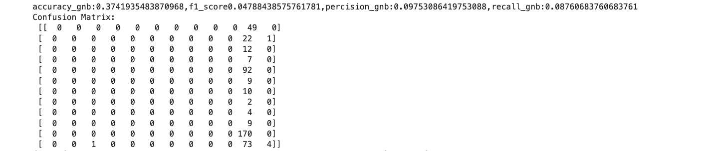
4. Categorical Naive Bayes (CNB):
Handles categorical data directly.
Example: Classifying crops based on soil color or other categorical features.
Comparison:
Gaussian NB is best for continuous data, while Multinomial NB and Bernoulli NB are better suited for discrete or binary data.
Categorical NB is specifically designed for categorical features, making it ideal for datasets with non-numeric attributes.
(b) Data Prep:
1. Labeled Data: The dataset is labeled.
2. Train-Test Split: The data is split into training and testing sets to evaluate model performance. The split must be disjoint to avoid data leakage.
3. Data Types: Different Naive Bayes flavors require different data formats.
Gaussian NB: Continuous features.
Multinomial NB: Discrete features.
Bernoulli NB: Binary features.
Categorical NB: Categorical features.
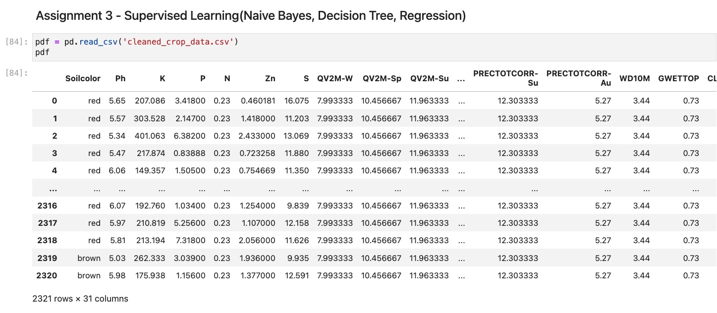
Link to the data prepared
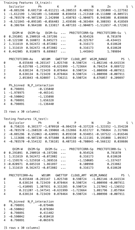
Image of the dataframe used.Dataframe too long to fit in this image.
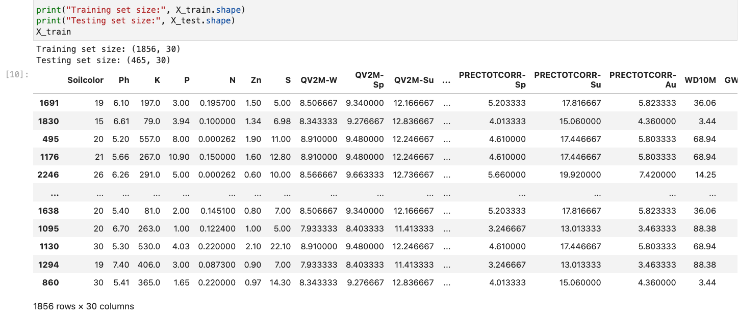
Training Dataframe:(X_train)
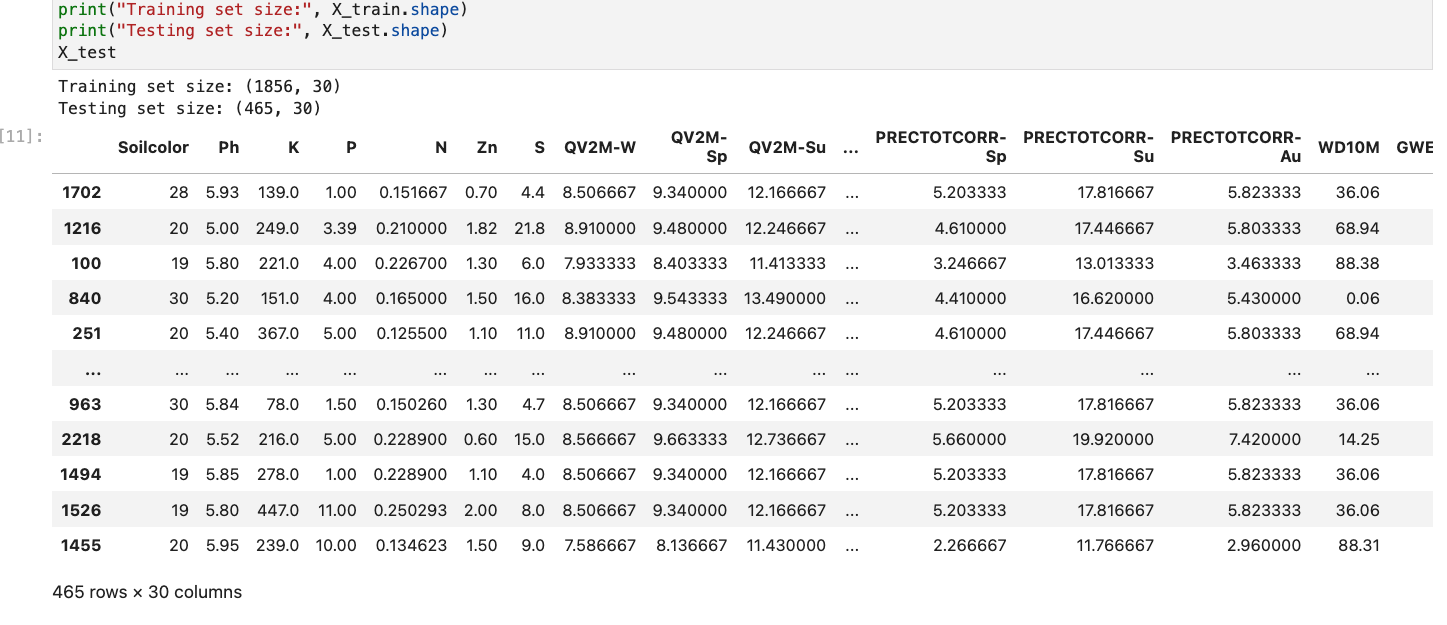
Testing Dataframe:(X_test)
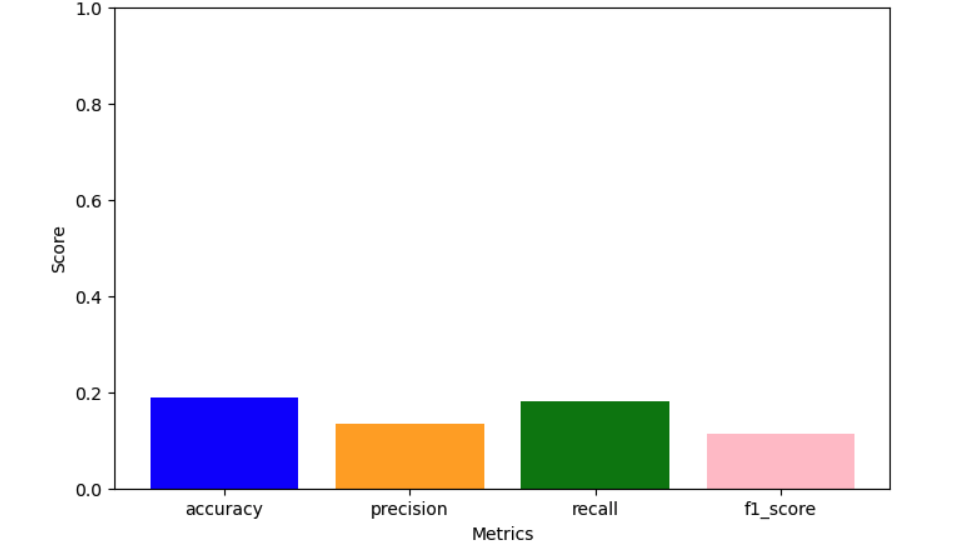
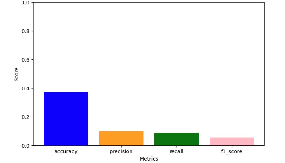
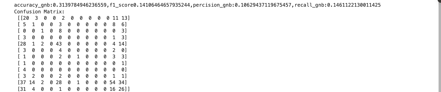
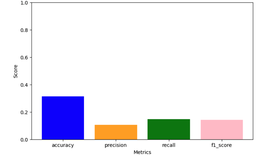
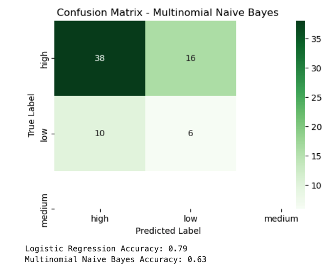
Accuracy Scores: Comparing the accuracy of the models.
Confusion Matrices: The confusion matrices for each model to visualize true positives, false positives, true negatives, and false negatives.
Observations:
1. Gaussian NB performs well with continuous features like pH and nutrient levels.
2. Multinomial NB is effective for discrete features like soil type.
3. Bernoulli NB.
4. Categorical NB is ideal for categorical features like soil color.
(e) Conclusions
Naive Bayes is a simple yet reliable classifier. It would be fine if we have the assumption of independence. Gaussian NB was suitable for continuous features, and Multinomial NB was suitable for discrete features, while Categorical NB was suitable for categorical features.
The models can be utilized to classify crop suitability based on soil and climate information to help farmers make intelligent decisions.
Supervised learning: Decision Trees
(a) Overview
Decision Trees (DTs) are a classification as well as regression method used in supervised learning. DTs partition the data according to feature values and construct a tree-based model. DTs are interpretable in nature and are able to process categorical as well as continuous data.
Main Ideas:
Gini Index: This is a measure of a node's impurity. In Gini, lower is desirable.
Entropy: It quantifies the randomness of information. Low entropy implies good splits.
Information Gain: The reduction of entropy after a split. The greater the information gain, the better the split.
Example of Gini and Information Gain:
I choose "Barley" and "Bean".
Gini Index before split: 0.5.
Gini Index after split: 0.2
Information Gain = 0.5 - 0.2 = 0.3.
Infinite Trees:
We can generate an unlimited number of trees by repeatedly partitioning the data. This will result in overfitting. We can prevent this by limiting tree depth or pruning.
(b) Data Prep:
Using the same dataset as Naive Bayes.
Spliting the data into training and testing sets.
Ensure the split is disjoint to avoid data leakage.
Image of the dataframe used.Dataframe too long to fit in this image.
1. Accuracy Scores: Comparing the accuracy of the trees.
2. Confusion Matrices: Displaying the confusion matrices for each tree.
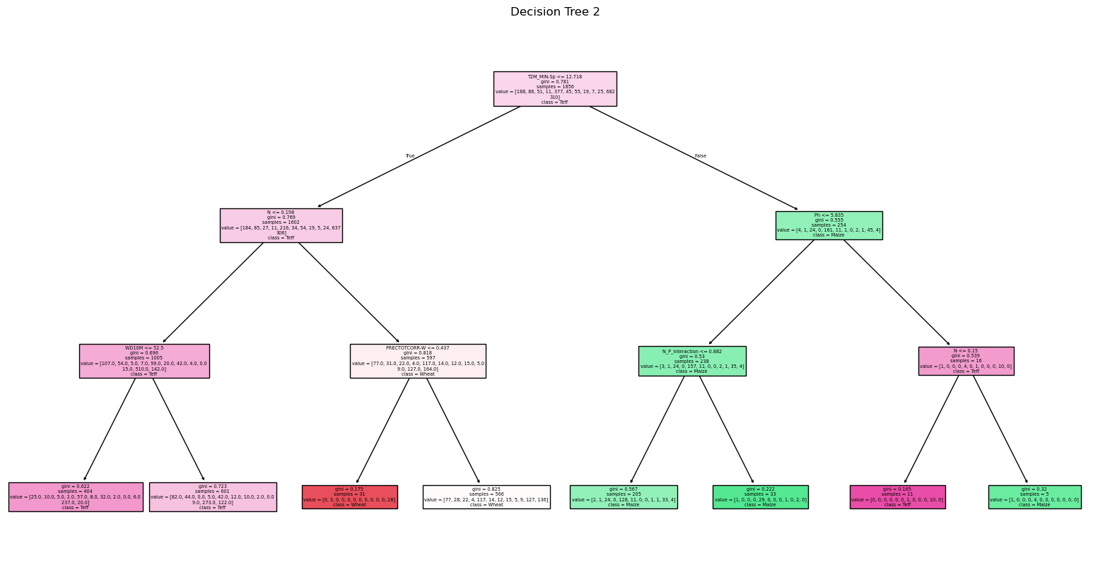
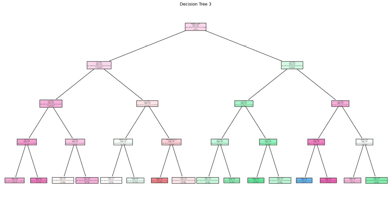
3. Tree Visualizations: Include visualizations of at least three different trees with different root nodes.
Observations:
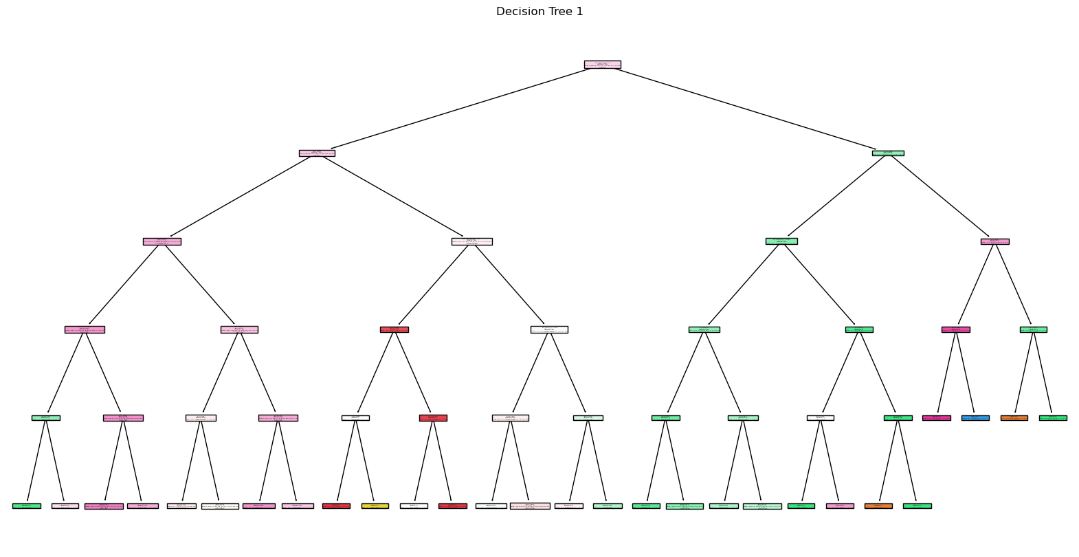
Decision Tree 1 (gini, max_depth=5)
Evaluation Metrics:
Decision tree plot:
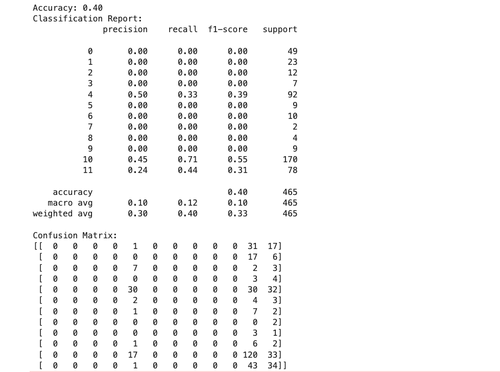
Decision Tree 2 (gini, max_depth=3)
Evaluation Metrics:
Decision tree plot:
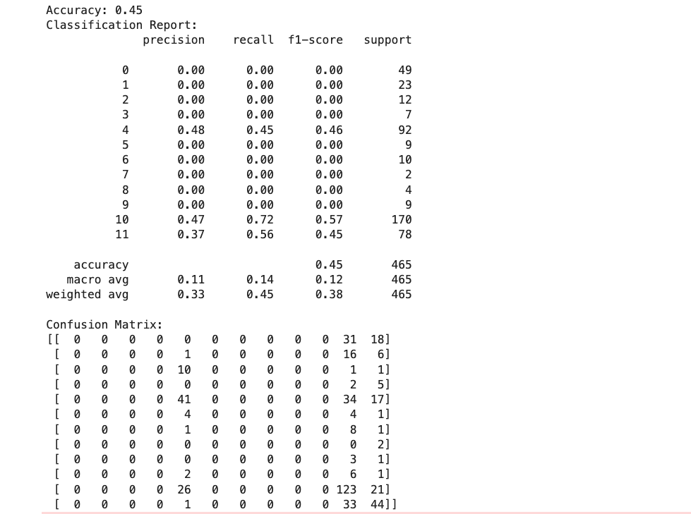
Decision Tree 3 (entropy, max_depth=4)
Evaluation Metrics:
Decision tree plot:
Max_depth =4 and criterion = entropy gave the highest accuracy.
(e) Conclusions
Decision Trees are explainable and are good for both continuous and categorical data. Decision Trees can be applied to discover the most influential features in crop suitability prediction.
They overfit, but it is possible to evade it by limiting tree depth or by pruning.
Supervised learning: Regression
(a) Define and explain linear regression.
Linear regression is a supervised learning model used to predict a continuous target variable. It illustrates the relationship between the target variable and one or more feature variables by fitting the data into a linear equation.
(b) Define and explain logistic regression.
Logistic regression is a supervised classifier for binary classification tasks. Logistic regression predicts a class probability through the use of the sigmoid function, which scales predictions onto the range 0 to 1.
(c) In how many ways are they alike, and in how many are they different?
Similarities:
Both are linear models.
Both utilize optimization routines to reduce loss functions.
Differences:
Linear regression predicts continuous values, but logistic regression predicts probabilities in classification.
Logistic regression uses the sigmoid function but linear regression does not.
(d) Does logistic regression use the Sigmoid function? Why?
Yes, logistic regression uses the sigmoid function to map predictions onto probabilities between 0 and 1. The sigmoid function ensures that the output can be understood as a probability.
(e) Explain how maximum likelihood is connected to logistic regression.
Logistic regression uses maximum likelihood estimation (MLE) to find parameters that maximize the likelihood of observed data. MLE guarantees the model's prediction is as close to the true data as possible.
Simple comparision of all 3 models:
1. Naive Bayes: Performs well with categorical and discrete features.
2. Decision Trees: Effective for both categorical and continuous data but prone to overfitting.
3. Logistic Regression: Ideal for binary classification tasks with continuous features.
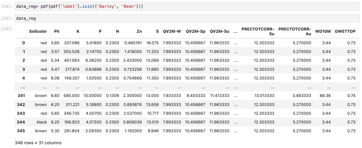
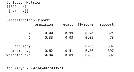
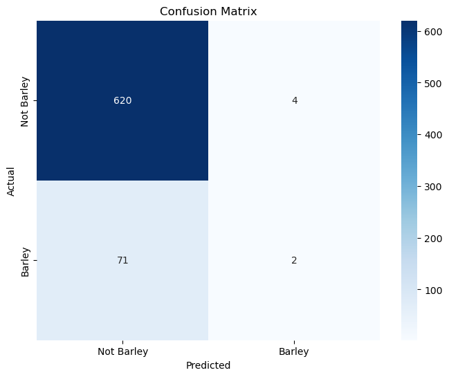
Coding: Comparing Logistic regression analysis and Multinomial Naive Bayes Classifiers
Image of the updated dataframe of two labels (Beans and Barley).
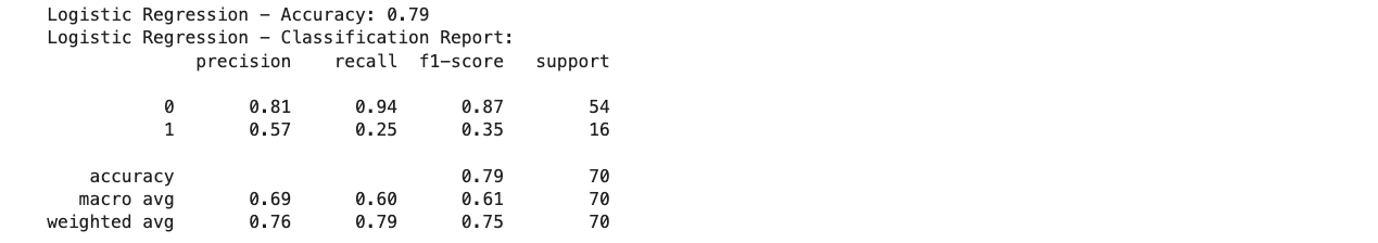
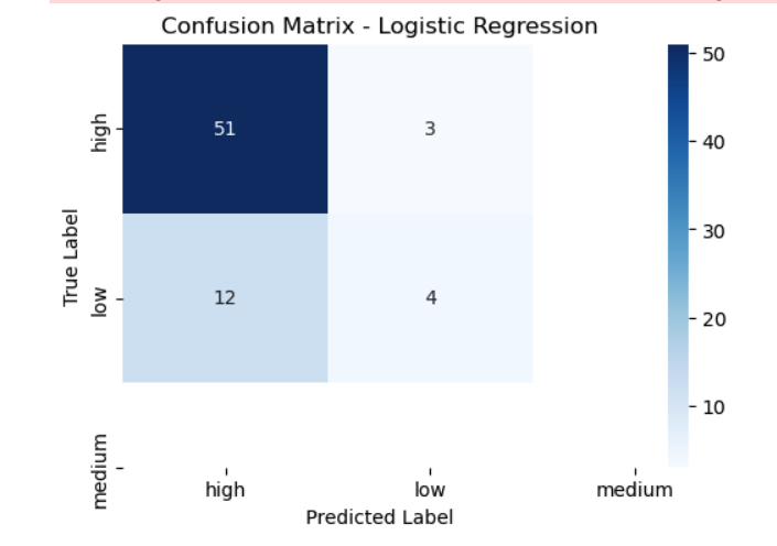
1.Logistic regression for updated 2 label dataset: Accuracy, classification report and confusion matrix below.
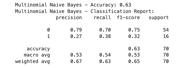
2. Naive bayes for updated 2 label dataset: Accuracy, classification report and confusion matrix below.
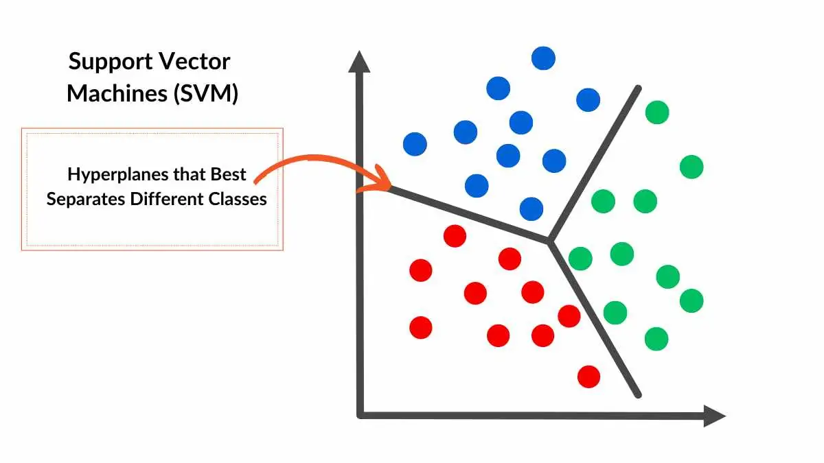
Supervised: Support Vector Machine
Overview
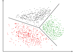
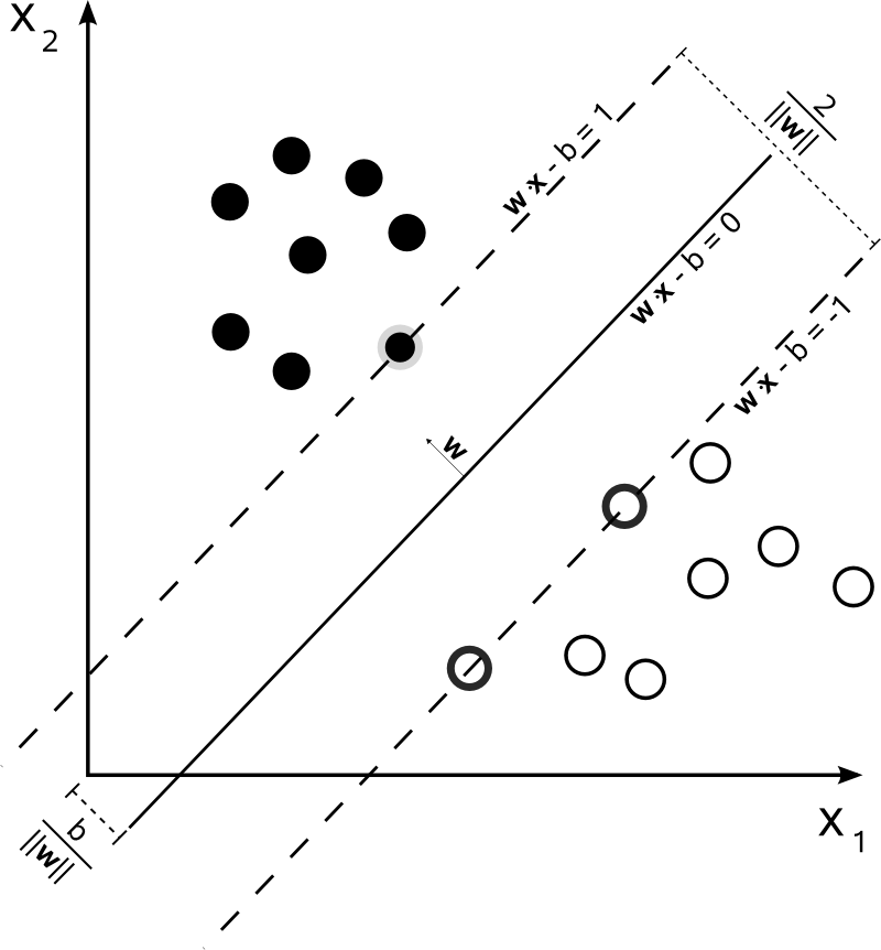
Support Vector Machines (SVMs) are a machine classification and regression learning algorithm that is supervised in nature. The primary task of SVMs is to find the optimal hyperplane that maximally separates data points of two classes in an N-dimensional space. The hyperplane is chosen based on maximizing the margin, i.e., the distance of the hyperplane from the nearest data points of either class, which is called support vectors. Through margin optimization, SVMs achieve improved generalization to novel data.
Why SVMs are Linear Separators?
SVMs are linear separators in the sense that they attempt to find a straight line (in 2D) or hyperplane (in more dimensions) which classifies the data into distinct classes. For linearly separable data, this hyperplane can be employed for complete separation of classes. However, for non-linearly separable data, SVMs use a kernel trick to project the data into higher dimensions where it can find a linear separator.
The Role of Kernel and Dot Product
The kernel function is a mathematically neat utility which finds the similarity between two points in the feature space after transformation but without the actual transformation taking place. Dot product is central to the kernel because it finds the similarity of two vectors, and this on which the entire kernel rests. For example, in the polynomial kernel, dot product is taken to a power such that non-linear relationships may be obtained.
Example:
Given 2D Point
Let’s take a 2D point:
x
=
(
x
1
,
x
2
)
=
(
2
,
3
)
x=(x
1
,x
2
)=(2,3)
Step 1: Expanded Polynomial Terms
For
d
=
2
d=2
, the polynomial kernel expands the input into:
A constant term:
1
1
The original features:
x
1
,
x
2
x
1
,x
2
The squared terms:
x
1
2
,
x
2
2
x
1
2
,x
2
2
The interaction term:
x
1
⋅
x
2
x
1
⋅x
2
Step 2: Transformed Point
Using the polynomial kernel with
r
=
1
r=1
and
d
=
2
d=2
:
ϕ
(
x
)
=
(
1
,
x
1
,
x
2
,
x
1
2
,
x
2
2
,
x
1
⋅
x
2
)
ϕ(x)=(1,x
1
,x
2
,x
1
2
,x
2
2
,x
1
⋅x
2
)
Substituting
x
1
=
2
x
1
=2
and
x
2
=
3
x
2
=3
:
ϕ
(
x
)
=
(
1
,
2
,
3
,
2
2
,
3
2
,
2
⋅
3
)
ϕ(x)=(1,2,3,2
2
,3
2
,2⋅3)
Calculating the values:
ϕ
(
x
)
=
(
1
,
2
,
3
,
4
,
9
,
6
)
ϕ(x)=(1,2,3,4,9,6)
Thus, the 2D point
(
2
,
3
)
(2,3)
is transformed into the 6D point
(
1
,
2
,
3
,
4
,
9
,
6
)
(1,2,3,4,9,6)
.
No, The purpose of this split is to ensure that the model is trained on one subset of the data (the training set) and evaluated on a different subset (the testing set). This separation is essential for assessing how well the model generalizes to unseen data.
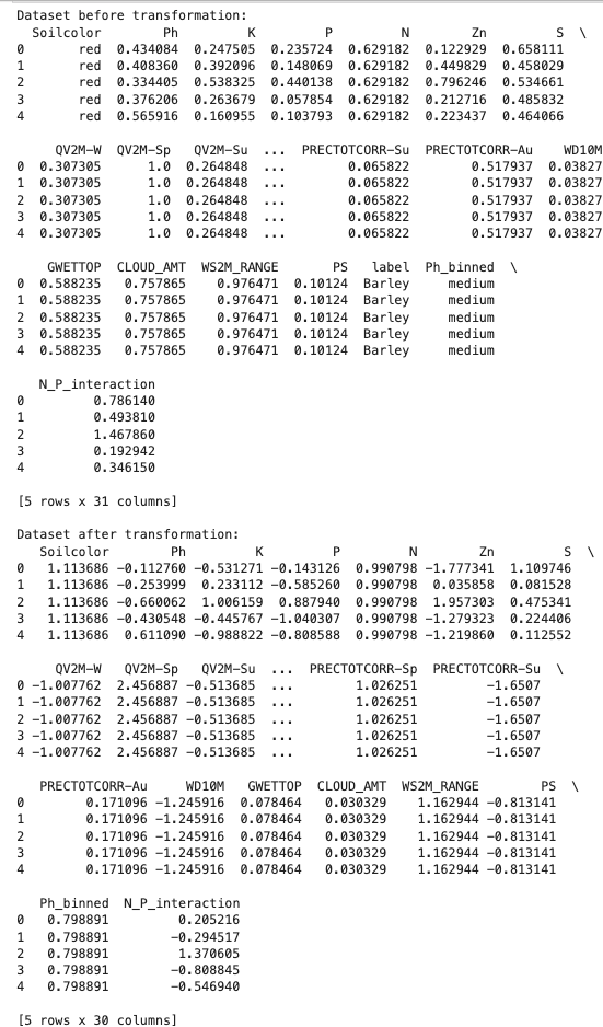
Data before and after transformation
- I split the training and testing parts in 70/30 ratio
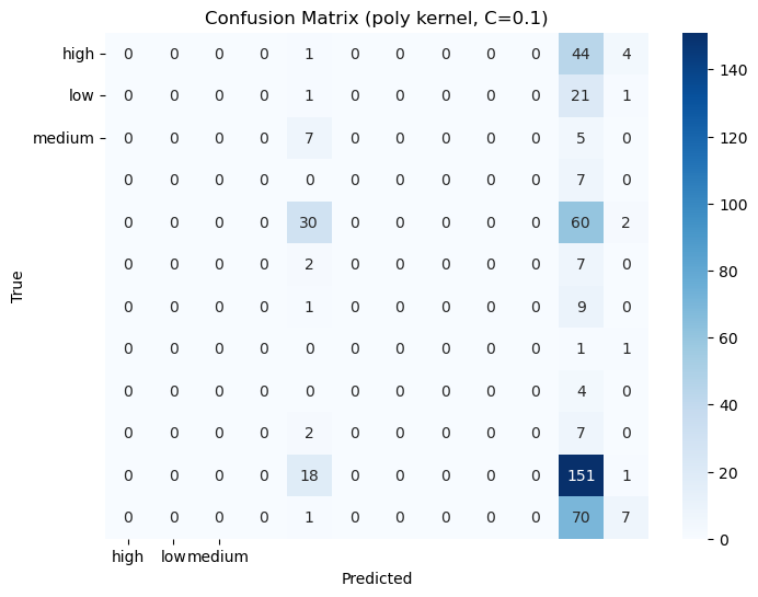
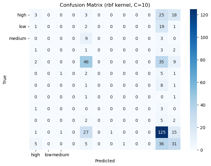
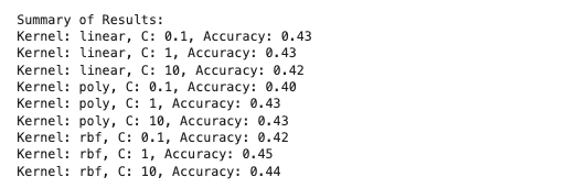
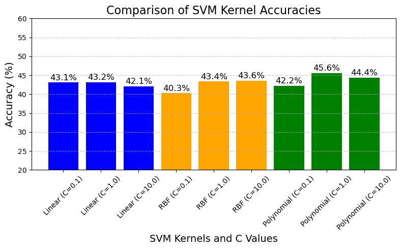
Three different Kernels with (linear, poly, rbf )3 differen C values(0.1, 1, 10)
Discussion: Almost every configuration gave the same result on this dataset.
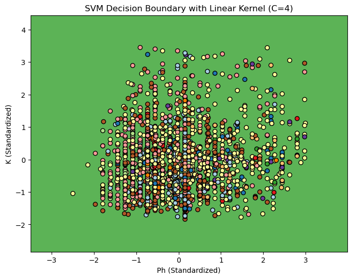
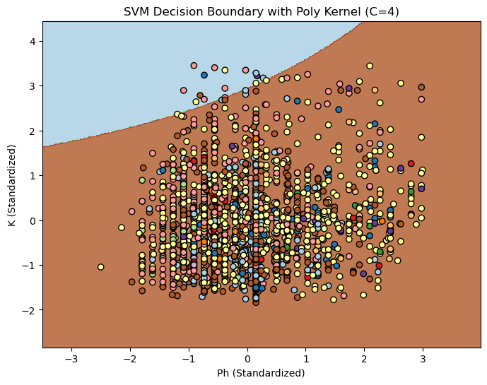
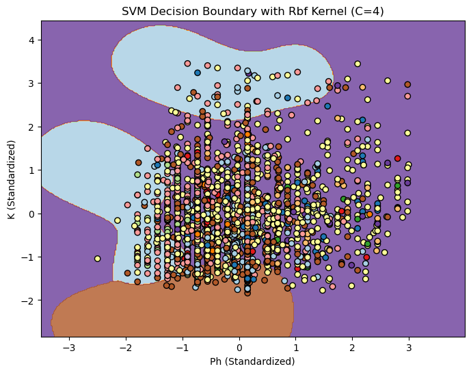
Decision Boundary SVM for C=4
Linear Ploy RBF
Ensembling Methods
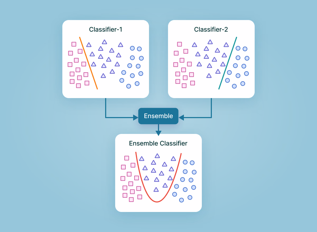
What is Ensemble Learning
A machine learning technique called ensemble learning combines the results of several models (also called "weak learners" or "base models") to produce a more robust and accurate model. Combining the outputs of different models is thought to improve generalisation, reduce mistakes, and produce better prediction performance than separate models.
The premise behind ensemble learning is that it is possible to take use of the differences between the basic models. While each model has its own advantages and disadvantages, when combined, they work in concert to produce predictions that are stronger and more reliable.
How this code applies to my project
Ensemble learning can be applied to your smart crop recommendation system to increase forecast accuracy and resilience. Combining several models (such as Random Forest, KNN, and Decision Tree) allows the system to minimise the drawbacks of each model while utilising its advantages. A more accurate and dependable recommendation system is produced by the Perceptron, which functions as a meta-model and learns the best weights to combine the basic models' predictions.
For example:
Tree: May overfit, but captures basic choice limits.
KNN: Has trouble with high-dimensional data but does well with local patterns.
Random Forest: May need more processing power, but it reduces overfitting and captures intricate patterns.
Results obtained with ensembling
The ensemble model combines the strengths of the base models and achieves higher accuracy than any individual model.
The Perceptron optimizes the weights of the base model predictions, ensuring that the final output is robust and reliable.
Brief of my ensemble approach
Ensemble learning is used which integrates several machine learning models to increase prediction accuracy and robustness. In particular, the project makes use of three foundational models:
A straightforward, interpretable model that divides data according to feature thresholds is called a decision tree classifier.
The K-Nearest Neighbours (KNN) algorithm is a distance-based algorithm that makes predictions based on the nearest neighbours' majority class.
An ensemble of decision trees called the Random Forest Classifier enhances generalisation and lessens overfitting.
A Perceptron Neural Network, which serves as a meta-model to determine the ideal weights for merging the base models' predictions, is used to integrate these models. This strategy makes sure that each model's advantages are maximised while reducing its disadvantages.
Numerical features with different scales
Categorical variables (Soil color, Ph_binned)
Mixed data types requiring preprocessing
Data after transformation:
Standardized numerical features (mean=0, std=1)
Encoded categorical variables
Engineered features (e.g., N_P_interaction)
Classification Report & Confusion matrix:
Results obtained: This new crop recommendation model utilized multiple machine learning models to accurately predict which crops are best suited for specific growing conditions. The system achieves an impressive accuracy of approximately 90%, indicating its effectiveness in making reliable crop recommendations. Key findings reveal that soil characteristics are the most significant factors influencing crop suitability, while weather patterns also play a crucial role. The system demonstrates versatility across various crop types, providing benefits such as improved resource utilization and a reduced risk of crop failure. However, it faces limitations, including a small dataset size of only 21 samples, limited seasonal data, and regional specificity, which may affect its generalizability.
Conclusions
The development of an intelligent crop recommendation system based on machine learning reiterates the transformational potential of data-related technologies in agriculture today. This paper illustrates the ability of intelligent algorithms, powered by the interaction of climatic conditions, weather forecasts, and types of soils, to inform the farmers in a better manner. It reduces farming activity complexities, enhances productivity, and enhances sustainability. It provides farmers with timely information to select the best possible crops according to their specific conditions, thereby improving productivity without wasting resources.
Most likely, the single most significant conclusion of this research is awareness regarding soil-climate-crop performance relationships. Experience-based traditional agricultural practices or traditional trends are insufficient in the wake of climate change at a rapid pace and degradation of soils. Machine learning, on the other hand, excels at uncovering concealed patterns in complex sets of data. To illustrate, it can map the influence of soil pH level, nutrient status, and climate patterns on harvest yield. This type of information is invaluable for farmers, who can make sensible, data-based decisions that return maximum yields for minimum risk.
The capacity of machine learning algorithms to learn and react to farm challenges is another important lesson. Various techniques, such as clustering, association rule mining, and supervised learning algorithms, were experimented in this research. Each one has strengths and weaknesses, but together they form a robust system that is able to handle the complexities of actual agriculture. For example, clustering might group similar soil types together, while supervised learning might figure out which crops are best suited for any given mix of conditions. This synergy makes the system comprehensive as well as adaptive.
Also, the system is agricultural sustainability-oriented. In that it recommends crops suitable for the situation at hand, it avoids overutilization of resources like water and fertilizers. Not only does this conserve resources, but also it avoids environmental degradation through cultivation. More so, weather sensitivity of the system encourages water conservation and assists farmers with adaptation to changing climatic factors. All these are aligned with global initiatives for promoting sustainable agriculture practice.
Lastly, this research validates the ability of machine learning to revolutionize agriculture and address some of the most pressing problems in the world. It envisions a world where productivity and sustainability are not opposing goals but complementary ones. Through technology and data, the system supports flourishing agricultural communities and world food security. This use of machine learning in farming is a giant step towards a more intelligent, sustainable future.
Once again thanks to Dr.Gates for providing this opportunity to explore ML through the course.